edgeListToCurve

Below is a demonstration of the features of the edgeListToCurve function

Syntax
Description
Examples
Getting indices for a single boundary curve
Getting indices for a multiple boundary curves

clear; close all; clc;

Syntax

[indList]=edgeListToCurve(E);

Description

This function converts the nx2 edges array E, which should define a single curve, to an ordered list of mx1 indices indList for that curve. Note that iff the edges define a closed curve the first and last indices in the ordered list are the same and therefore repeated.

Examples

Plot settings

markerSize=40;
lineWidth=4;
fontSize=25;

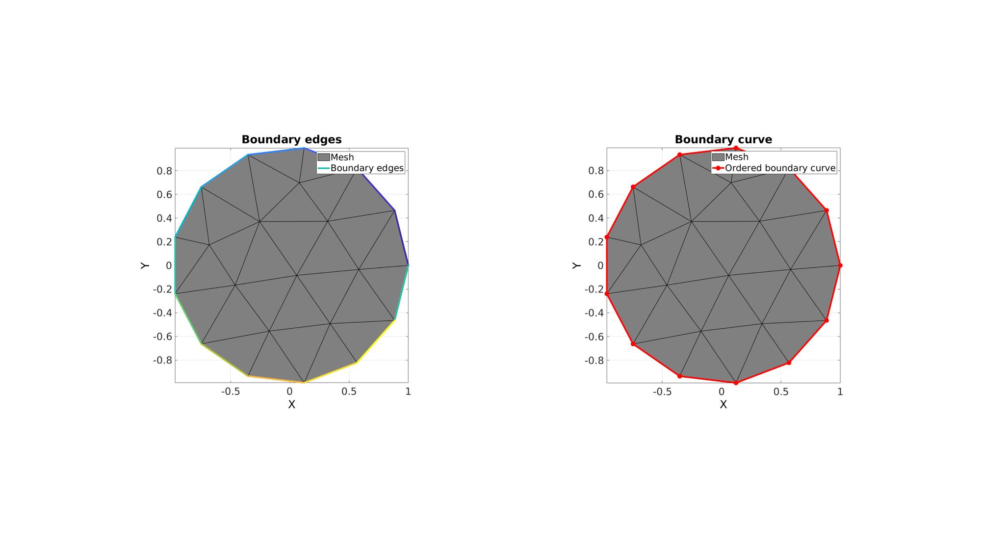
Getting indices for a single boundary curve

Creating example geometry

t=linspace(0,2*pi,50); t=t(1:end-1); %Angles
V1=[cos(t(:)) sin(t(:))];

%Desired point spacing
pointSpacing=0.5;

[F,V]=regionTriMesh2D({V1},pointSpacing,1,0);

Get boundary edges

Eb=patchBoundary(F,V);

Use edgeListToCurve to get curve indices

indList=edgeListToCurve(Eb);

Visualize example mesh and boundary edges/curves

cFigure;
subplot(1,2,1); hold on;
title('Boundary edges','FontSize',fontSize)
hp1=gpatch(F,V,'kw','k',1,1);
hp2=gpatch(Eb,V,'none',(1:1:size(Eb,1))',1,lineWidth);
legend([hp1 hp2],{'Mesh','Boundary edges'});
axisGeom(gca,fontSize); view(2);

subplot(1,2,2); hold on;
title('Boundary curve','FontSize',fontSize)
hp1=gpatch(F,V,'kw','k',1,1);
hp2=plotV(V(indList,:),'r.-','MarkerSize',markerSize,'LineWidth',lineWidth);
legend([hp1 hp2],{'Mesh','Ordered boundary curve'});
axisGeom(gca,fontSize); view(2);

drawnow;

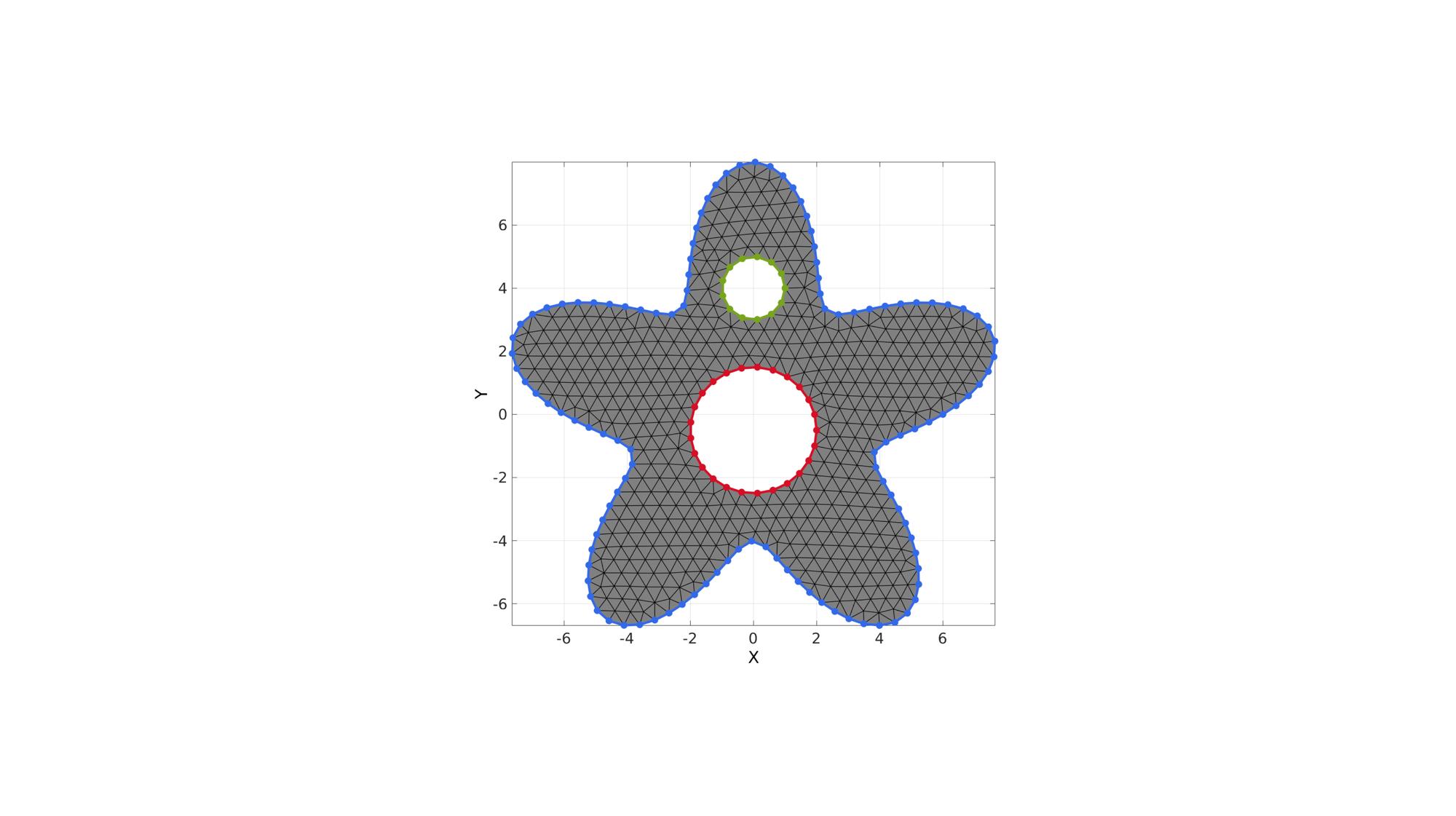
Getting indices for a multiple boundary curves

Creating example geometry with multiple boundary sets

%Boundary 1
ns=150;
t=linspace(0,2*pi,ns);
t=t(1:end-1);
r=6+2.*sin(5*t);
[x,y] = pol2cart(t,r);
V1=[x(:) y(:)];

%Boundary 2
[x,y] = pol2cart(t,ones(size(t)));
V2=[x(:) y(:)+4];

%Boundary 3
[x,y] = pol2cart(t,2*ones(size(t)));
V3=[x(:) y(:)-0.5];

%Defining a region
regionCell={V1,V2,V3}; %A region between V1 and V2 (V2 forms a hole inside V1)

plotOn=1; %This turns on/off plotting

%Desired point spacing
pointSpacing=0.5;

[F,V]=regionTriMesh2D(regionCell,pointSpacing,1,0);

Get boundary edges

Eb=patchBoundary(F,V);

Use grouping to "seperate" boundary sets

optionStruct.outputType='label';
G=tesgroup(Eb,optionStruct);

cFigure; hold on;
gpatch(F,V,'kw','k',1,1);
axisGeom(gca,fontSize); view(2);

plotColors=gjet(max(G(:)));
for q=1:1:max(G(:))

    E_now=Eb(G==q,:);

    plotV(V(E_now,:),'b.','markersize',25);

    [indListNow]=edgeListToCurve(E_now);

    hp=plotV(V(indListNow,:),'b.-','MarkerSize',markerSize,'LineWidth',lineWidth);
    hp.Color=plotColors(q,:);

end

drawnow;

GIBBON www.gibboncode.org

Kevin Mattheus Moerman, [email protected]

GIBBON footer text

License: https://github.com/gibbonCode/GIBBON/blob/master/LICENSE

GIBBON: The Geometry and Image-based Bioengineering add-On. A toolbox for image segmentation, image-based modeling, meshing, and finite element analysis.

This program is free software: you can redistribute it and/or modify it under the terms of the GNU General Public License as published by the Free Software Foundation, either version 3 of the License, or (at your option) any later version.

This program is distributed in the hope that it will be useful, but WITHOUT ANY WARRANTY; without even the implied warranty of MERCHANTABILITY or FITNESS FOR A PARTICULAR PURPOSE. See the GNU General Public License for more details.