hessianScalar

Below is a demonstration of the features of the hessianScalar function See also: gradient,|hessian|,|jacobian|,|cellEig|.

Syntax
Description
Examples
1D Hessian on vector
2D Hessian on a matrix (e.g. an image)
The cell output option

clear; close all; clc;

Syntax

H=hessianScalar(M,voxelSize,cellOpt);

Description

This function computes the Hessian matrix of the scalar function U for each point in U. U may be a vector, a 2D matrix or a 3D matrix. The vector v denotes the points spacing between the data entries in U. If v is not supplied the spacing is assumed to be homogeneous and unity. If the input is n dimensional array consisting of m entries then the output is a matrix (if cellOpt==0) the size of mx(n^2) (whereby the colum entries define the entries in a Hessian matrix and row entries relate to elements in the input array). If cellOpt==1 then the output is reformed into a cell array that matches the size of the input aray. Each cell entry then contains the nxn Hessian matrix.

Examples

Plot settings

faceAlpha1=1;
faceAlpha2=0.3;
fontSize=10;
markerSize=25;
edgeWidth=1;
edgeColor='k';
cMap=gray(250);

1D Hessian on vector

%A random vector
M=randn(10,1)

%Compute Hessian
H=hessianScalar(M,[],0)

2D Hessian on a matrix (e.g. an image)

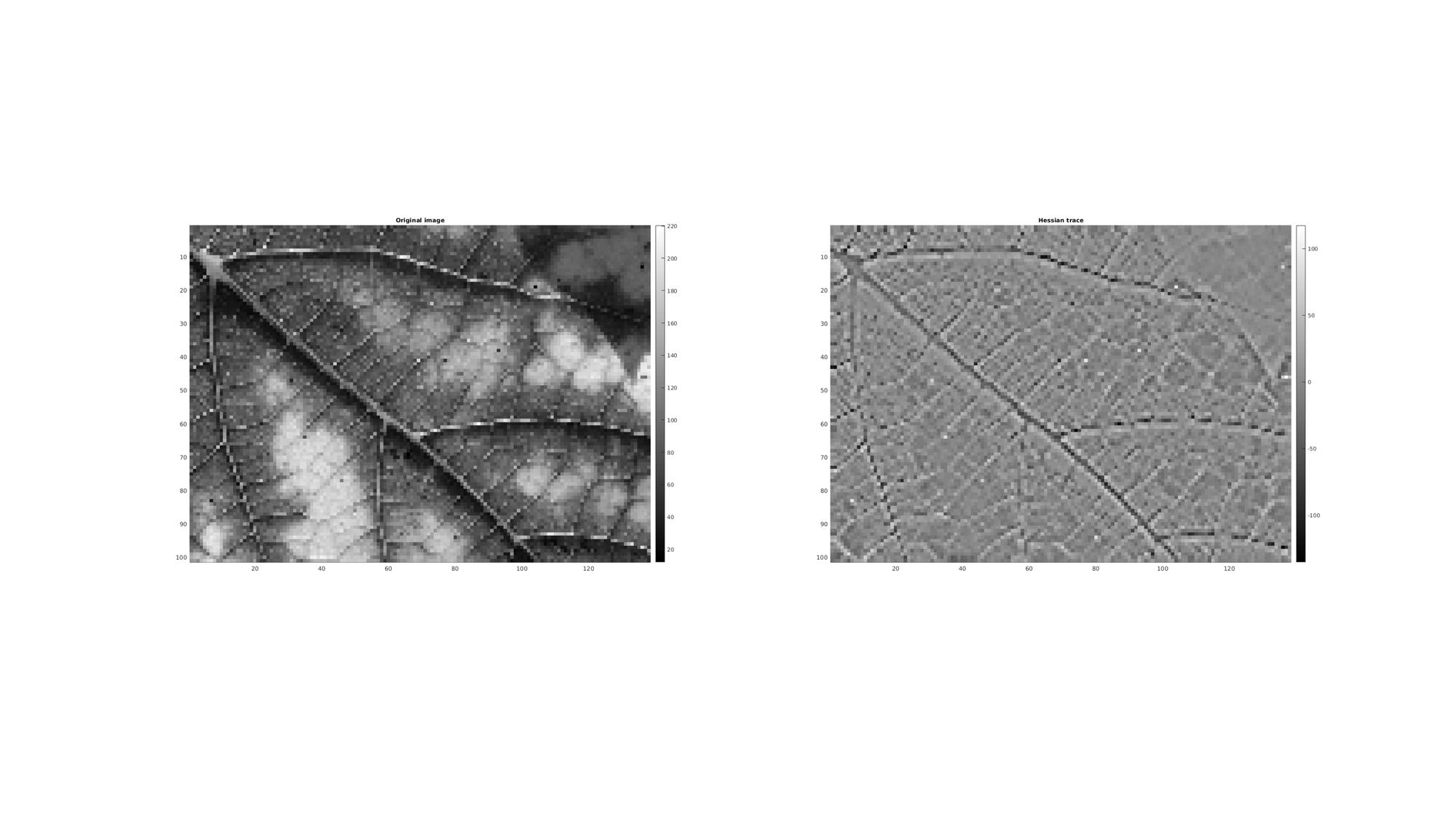
Below an example is shown for the Hessian of an image.

Load example image

%Set main folder
defaultFolder = fileparts(fileparts(mfilename('fullpath')));
pathName=fullfile(defaultFolder,'data','PICT');
loadName=fullfile(pathName,'leaf1.jpg'); %Load name
M=mean(double(importdata(loadName)),3); %Import and conver to grayscale
n=4;
M=M(1:n:end,1:n:end);

Computing the Hessian of the image

voxelSize=[1 1];
cellOpt=0;
H=hessianScalar(M,voxelSize,cellOpt);

In the above example the third input, cellOpt, was set to zero this leads to a m x (n^2) array whereby the colum entries define the entries in a Hessian matrix and row entries relate to elements in the input array. In this case a Hessian trace image can be computed as:

Mh_trace=reshape(H(:,1)+H(:,end),size(M)); %Compute trace for visualization

Visualize results

cFigure;

subplot(1,2,1); hold on;
title('Original image','fontSize',fontSize);
imagesc(M);
axis equal; axis tight; axis ij;
colormap(cMap); colorbar;

subplot(1,2,2); hold on;
title('Hessian trace','fontSize',fontSize);
imagesc(Mh_trace);
axis equal; axis tight; axis ij;
colormap(cMap); colorbar;

drawnow;

The cell output option

Alternatively if cellOpt==1 then the output is reformed into a cell array that matches the size of the input aray. Each cell entry then contains the nxn Hessian matrix. However this requires a matrix to cell and reshape operation making this approach slower than when cellOpt==0. However after conversion to cell form each cell contains a Hessian matrix and computations on these matrices can be performed using the syntax: [B]=cellfun(@my_func,H,'UniformOutput',0); Where my_func is a suitable function for the Hessian matrices. For instance to computer a trace image one can use: [B]=cellfun(@trace,A,'UniformOutput',0); This form has also been created as a function, namely cellTrace, see below.

Computing the Hessian of the image

voxelSize=[1 1];
cellOpt=1;
H=hessianScalar(M,voxelSize,cellOpt);

Each cell contains a Hessian matrix, for example:

H{1,1}

ans =

   -0.6667   -6.6667
   -6.6667    3.0000

Compute a trace image using cellTrace function:

Mh_trace=cellTrace(H);

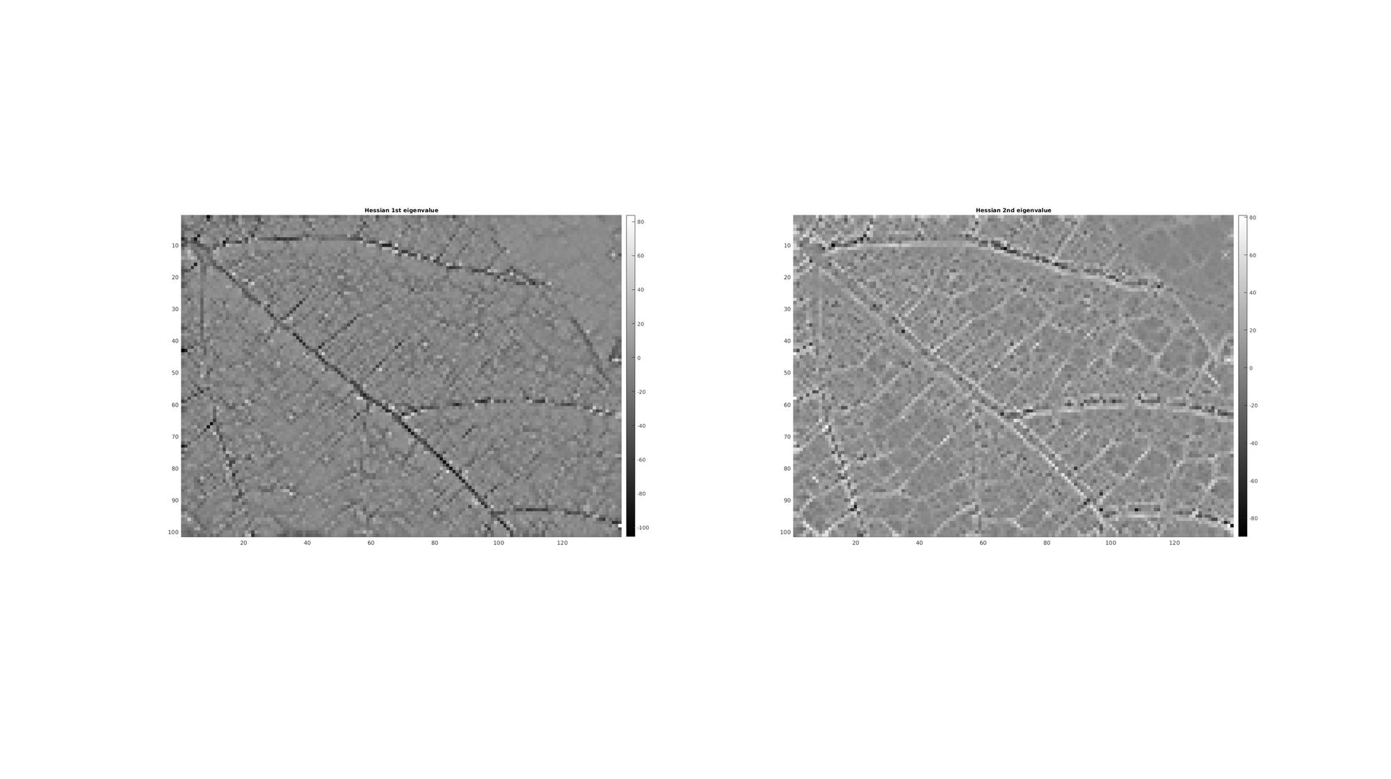
Computing eigenvalues using cellEig function:

[Mh_V,Mh_D]=cellEig(H);

%Get first and second eigenvalues
[Mh_D1]=cell2mat(cellfun(@(x) x(1,1) ,Mh_D,'UniformOutput',0));
[Mh_D2]=cell2mat(cellfun(@(x) x(2,2) ,Mh_D,'UniformOutput',0));

Visualize results

cFigure;

subplot(1,2,1); hold on;
title('Hessian 1st eigenvalue','fontSize',fontSize);
imagesc(Mh_D1);
axis equal; axis tight; axis ij;
colormap(cMap); colorbar;

subplot(1,2,2); hold on;
title('Hessian 2nd eigenvalue','fontSize',fontSize);
imagesc(Mh_D2);
axis equal; axis tight; axis ij;
colormap(cMap); colorbar;

drawnow;

GIBBON www.gibboncode.org

Kevin Mattheus Moerman, [email protected]

GIBBON footer text

License: https://github.com/gibbonCode/GIBBON/blob/master/LICENSE

GIBBON: The Geometry and Image-based Bioengineering add-On. A toolbox for image segmentation, image-based modeling, meshing, and finite element analysis.

This program is free software: you can redistribute it and/or modify it under the terms of the GNU General Public License as published by the Free Software Foundation, either version 3 of the License, or (at your option) any later version.

This program is distributed in the hope that it will be useful, but WITHOUT ANY WARRANTY; without even the implied warranty of MERCHANTABILITY or FITNESS FOR A PARTICULAR PURPOSE. See the GNU General Public License for more details.

You should have received a copy of the GNU General Public License along with this program. If not, see http://www.gnu.org/licenses/.