quiver3Dpatch

Below is a demonstration of the features of the quiver3Dpatch function

Plotting a vector
Defining vector lengths and colours
Example visualising coordinate system base vectors
Example for multidimensional image data 1: colormap driven vectors combined with RGB driven iso-surfaces
Example for multidimensional image data 2: RGB driven vectors combined with colormap driven iso-surfaces

clear; close all; clc;

Plot settings

cMap=jet(250);
faceAlpha1=1;
faceAlpha2=1;
edgeColor1='none';
edgeColor2='none';
cMap1=gjet(250);
cMap2=gray(250);
fontSize=15;

Plotting a vector

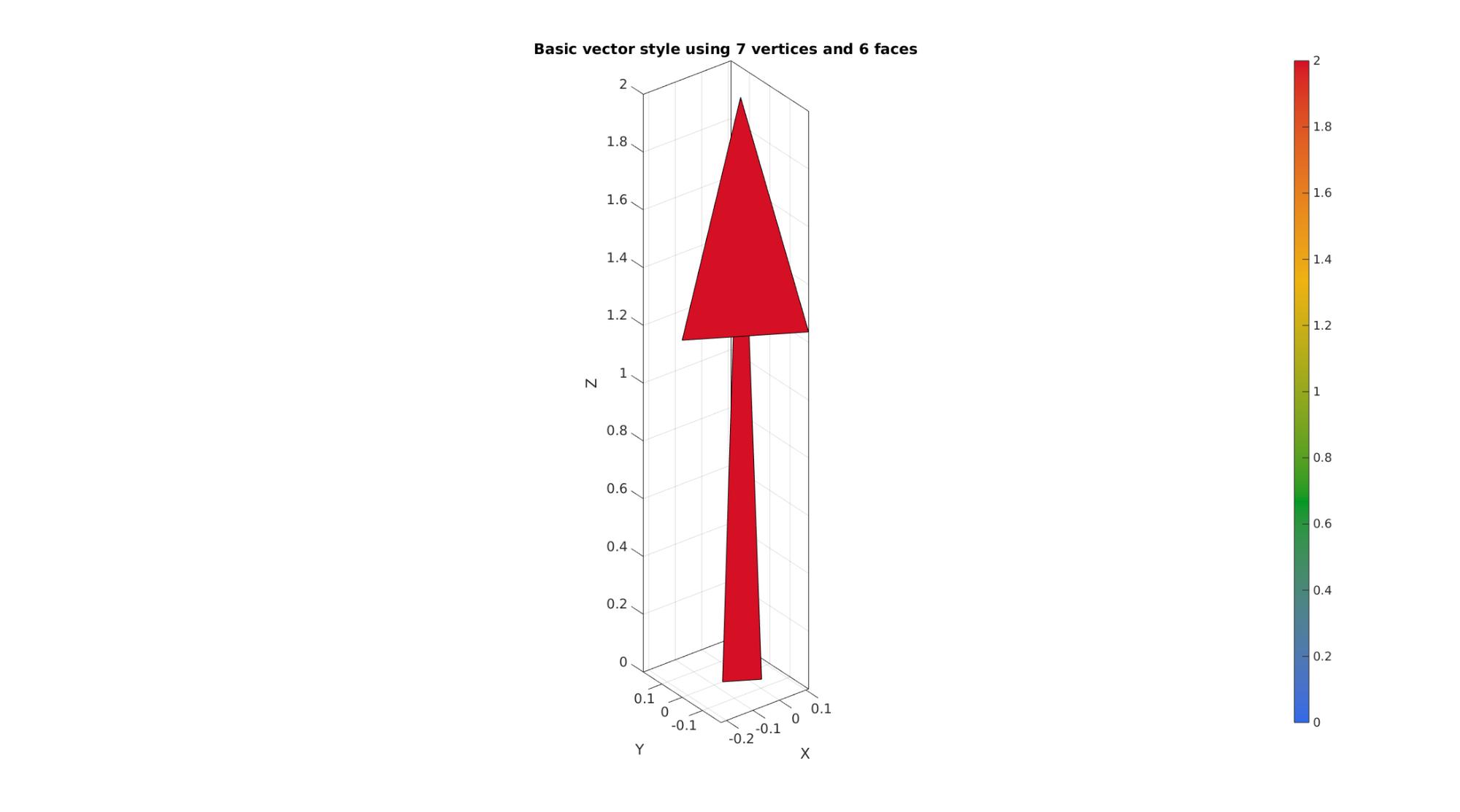
Below is a visualisation of the basec vector style

%Defining a single vector colinear with the Z-axis with length 2
X=0; Y=0; Z=0; %Vector origin (position vector components)
u=0; v=0; w=2; %Vector components
G=sqrt(u.^2+v.^2+w.^2); %Vector magnitude
cLim=[0 max(G(:))];
Cv=[]; %If empty then vector magnitude based scaling is used

a=[min(G(:)) max(G(:))]; %Arrow length scaling to magnitude range
[F1,V1,C1]=quiver3Dpatch(X,Y,Z,u,v,w,Cv,a);

cFigure;
title('Basic vector style using 7 vertices and 6 faces');
gpatch(F1,V1,C1);
colormap(cMap1); colorbar; clim(cLim);
axisGeom(gca,fontSize);
drawnow;

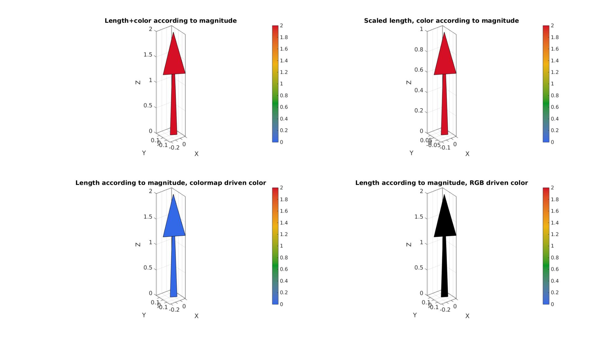
Defining vector lengths and colours

a=[min(G(:)) max(G(:))]; %Arrow length scaling to magnitude range
[F1,V1,C1]=quiver3Dpatch(X,Y,Z,u,v,w,Cv,a);

a=[1 1]; %Arrow length scaling min=1, max=1
[F2,V2,C2]=quiver3Dpatch(X,Y,Z,u,v,w,Cv,a);

a=[min(G(:)) max(G(:))]; %Arrow length scaling to magnitude range
Cv=zeros(size(X));
[F3,V3,C3]=quiver3Dpatch(X,Y,Z,u,v,w,Cv,a);

C4=cmaperise(C3,cMap2,cLim);

cFigure;
subplot(2,2,1);
title('Length+color according to magnitude');
gpatch(F1,V1,C1);
colormap(gca,cMap1); colorbar; clim(cLim);
axisGeom(gca,fontSize);

subplot(2,2,2);
title('Scaled length, color according to magnitude');
gpatch(F2,V2,C2);
colormap(gca,cMap1); colorbar; clim(cLim);
axisGeom(gca,fontSize);

subplot(2,2,3);
title('Length according to magnitude, colormap driven color');
gpatch(F3,V3,C3);
colormap(gca,cMap1); colorbar; clim(cLim);
axisGeom(gca,fontSize);

subplot(2,2,4);
title('Length according to magnitude, RGB driven color');
gpatch(F3,V3,C4);
colormap(gca,cMap1); colorbar; clim(cLim);
axisGeom(gca,fontSize);
drawnow;

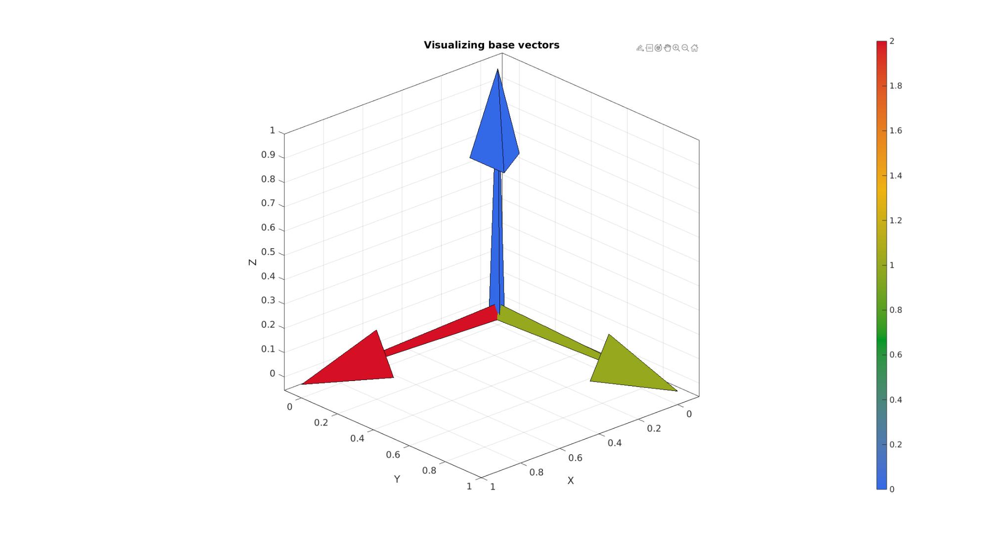
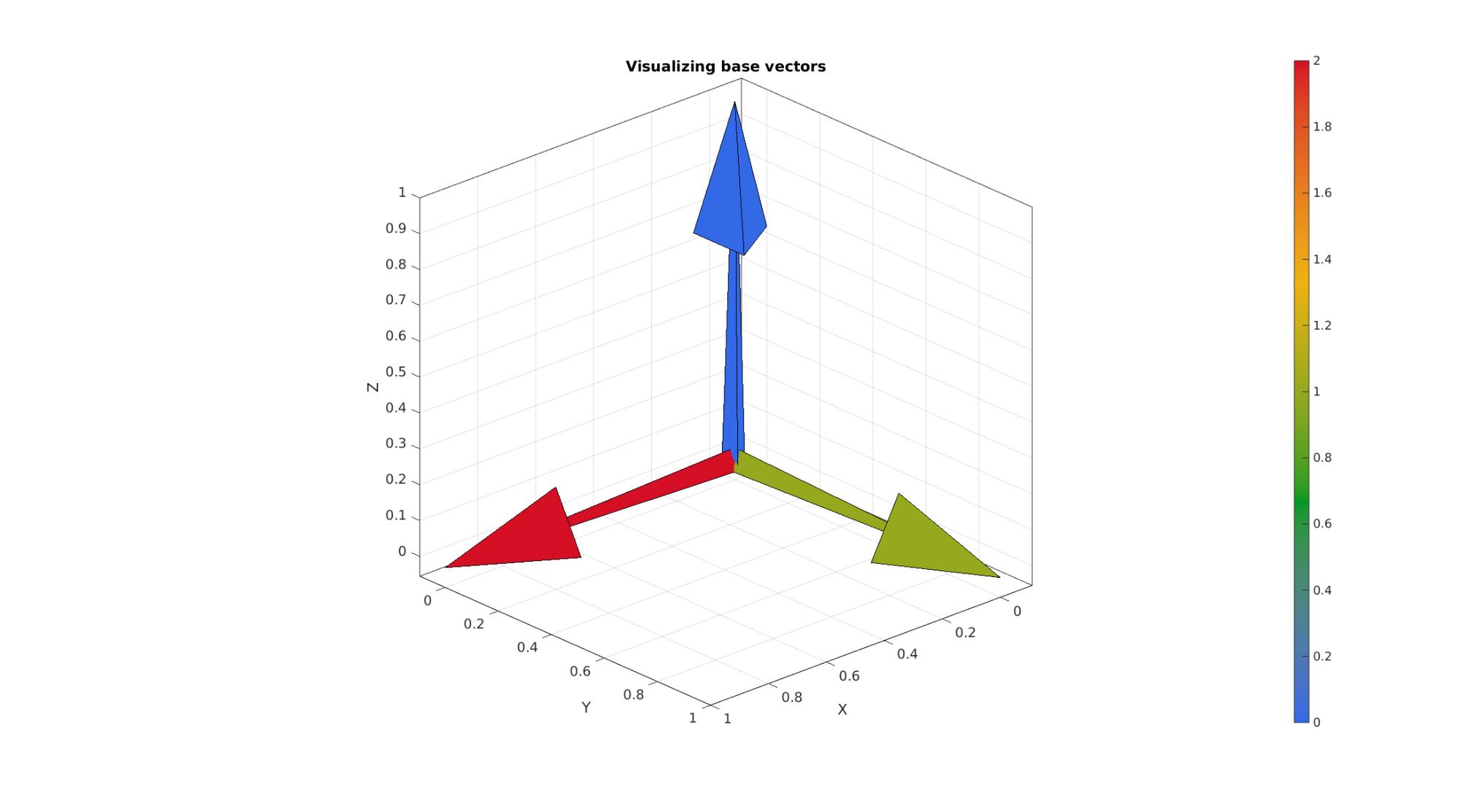
Example visualising coordinate system base vectors

originBasis1=[0 0 0];
E1=eye(3,3);
C1=[2 1 0];

originBasis2=[0 0 0];
E2=[2/3 -1/3  2/3; 2/3 2/3 -1/3; -1/3 2/3 2/3];
C2=[5 4 3];

[Fc1,Vc1,Cc1]=quiver3Dpatch(originBasis1(1)*ones(1,3), originBasis1(2)*ones(1,3), originBasis1(3)*ones(1,3),E1(:,1),E1(:,2),E1(:,3),C1',[1 1]);
[Fc2,Vc2,Cc2]=quiver3Dpatch(originBasis2(1)*ones(1,3), originBasis2(2)*ones(1,3), originBasis2(3)*ones(1,3),E2(:,1),E2(:,2),E2(:,3),C2',[1 1]);

cFigure;
title('Visualizing base vectors','FontSize',fontSize);
gpatch(Fc1,Vc1,Cc1,'k',1);
gpatch(Fc1,Vc1,Cc1,'k',0.5);
colormap(cMap1); colorbar; clim(cLim);
axisGeom(gca,fontSize); view([137.5,24]);
drawnow;

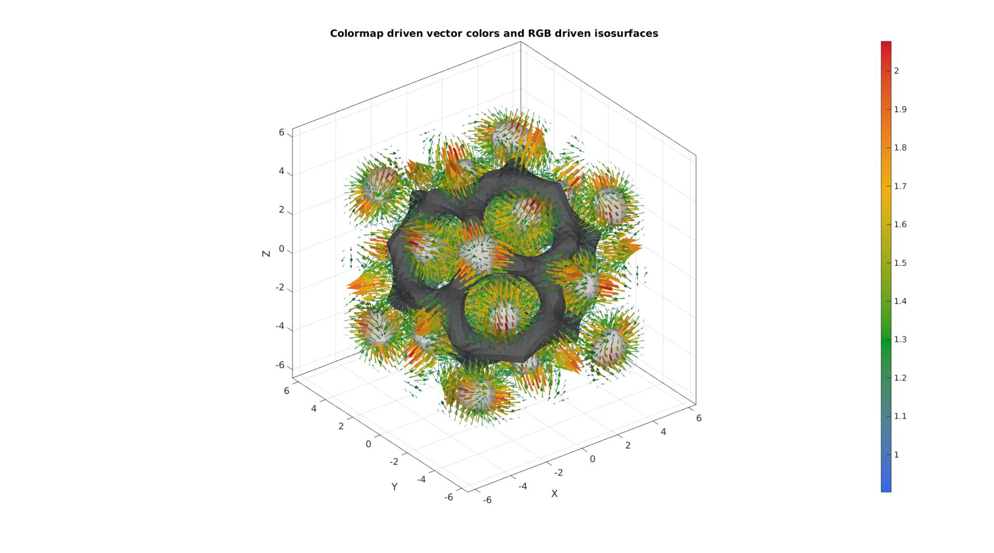
Example for multidimensional image data 1: colormap driven vectors combined with RGB driven iso-surfaces

Simulating 3D volume and vector data

n=27;
[X,Y,Z]=meshgrid(linspace(-4.77,4.77,n));
phi=(1+sqrt(5))/2;
M=2 - (cos(X + phi*Y) + cos(X - phi*Y) + cos(Y + phi*Z) + cos(Y - phi*Z) + cos(Z - phi*X) + cos(Z + phi*X));

Simulating vector data

%Vector data here based on the gradient of the image
[u,v,w] = gradient(M);
G=hypot(hypot(u,v),w); %Vector lenghts

%Iso-surface patch data to illustrate joint plotting
c_iso1=0; c_iso2=5;
[Fi1,Vi1,Ci1] = isosurface(X,Y,Z,M,c_iso1,M);
[Fi2,Vi2,Ci2] = isosurface(X,Y,Z,M,c_iso2,M);
a=[min(G(:)) max(G(:))]; %Arrow length scaling
L=G>0.9; %Logic indices for arrows
[Fv,Vv,Cv]=quiver3Dpatch(X(L),Y(L),Z(L),u(L),v(L),w(L),G(L),a);

cLim=[min(M(:)) max(M(:))]; %Colorbar limits
[Ci1n]=cmaperise(Ci1,cMap2,cLim);
[Ci2n]=cmaperise(Ci2,cMap2,cLim);

cFigure; hold on;
title('Colormap driven vector colors and RGB driven isosurfaces','FontSize',fontSize);
gpatch(Fv,Vv,Cv,edgeColor1,1);
gpatch(Fi1,Vi1,Ci1n,edgeColor2,faceAlpha2);
gpatch(Fi2,Vi2,Ci2n,edgeColor2,faceAlpha2);
colormap(cMap1); colorbar; clim([min(Cv(:)) max(Cv(:))]);
axisGeom(gca,fontSize); camlight headlight;
drawnow;

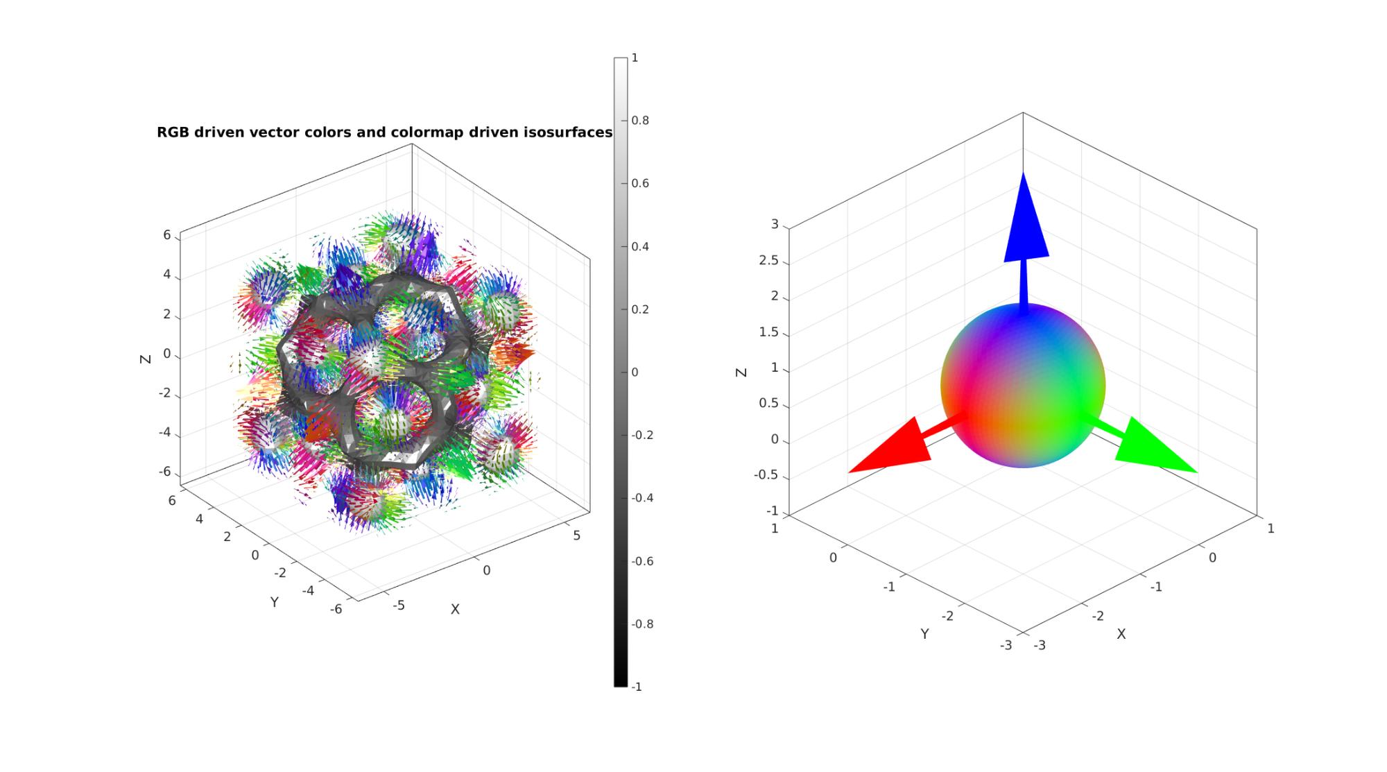
Example for multidimensional image data 2: RGB driven vectors combined with colormap driven iso-surfaces

Angle driven color can also be specified e.g. RGB values indicating vector angle

%Specifying angle dependant RGB type color
Xc=repmat(u(L),[6,1]); Yc=repmat(v(L),[6,1]); Zc=repmat(w(L),[6,1]);
Crgb=[Xc(:) Yc(:) Zc(:)];
M=sqrt(Crgb(:,1).^2+Crgb(:,2).^2+Crgb(:,3).^2);
Crgb=abs(Crgb./(M*ones(1,3))); %Normalising color

Defining a sphere to show the color mapping

[F,V,~]=geoSphere(4,1);
Xs=V(:,1); Ys=V(:,2); Zs=V(:,3);
C=[mean(Xs(F),2) mean(Ys(F),2) mean(Zs(F),2)]; %color for angles

The figure now demonstrates isosurfaces for the image data with overlain the gradient vectors coloured according to their direction

cFigure;
subplot(1,2,1);
xlabel('X','FontSize',fontSize);ylabel('Y','FontSize',fontSize);zlabel('Z','FontSize',fontSize);
title('RGB driven vector colors and colormap driven isosurfaces','FontSize',fontSize);

Cv=vecnormalize(Vv);

gpatch(Fv,Vv,Crgb,edgeColor1,1);
gpatch(Fi1,Vi1,Ci1,edgeColor2,faceAlpha2);
gpatch(Fi2,Vi2,Ci2,edgeColor2,faceAlpha2);

patch('Faces',Fv,'Vertices',Vv,'EdgeColor','none', 'FaceVertexCData',Crgb,'FaceColor','flat','FaceAlpha',1);
patch('Faces',Fi1,'Vertices',Vi1,'FaceColor','flat','CData',Ci1,'EdgeColor',edgeColor2,'FaceAlpha',faceAlpha2); hold on;
patch('Faces',Fi2,'Vertices',Vi2,'FaceColor','flat','CData',Ci2,'EdgeColor',edgeColor2,'FaceAlpha',faceAlpha2); hold on;
colormap(cMap2); colorbar; clim([min(Cv(:)) max(Cv(:))]);
axisGeom(gca,fontSize); camlight headlight;

subplot(1,2,2);
hp=gpatch(F,V,abs(C),'none',1);
DCM=eye(3,3);
origin=[0 0 0];
[Fa,Va,Ca]=quiver3Dpatch(origin(1)*ones(1,3), origin(2)*ones(1,3), origin(3)*ones(1,3),-DCM(:,1),-DCM(:,2),DCM(:,3),[],[3,3]);
hp2=gpatch(Fa,Va,repmat(eye(3,3),6,1),'none',1); hold on;

axisGeom(gca,fontSize); view(-45,30);
drawnow;

GIBBON www.gibboncode.org

Kevin Mattheus Moerman, [email protected]

GIBBON footer text

License: https://github.com/gibbonCode/GIBBON/blob/master/LICENSE

GIBBON: The Geometry and Image-based Bioengineering add-On. A toolbox for image segmentation, image-based modeling, meshing, and finite element analysis.

This program is free software: you can redistribute it and/or modify it under the terms of the GNU General Public License as published by the Free Software Foundation, either version 3 of the License, or (at your option) any later version.

This program is distributed in the hope that it will be useful, but WITHOUT ANY WARRANTY; without even the implied warranty of MERCHANTABILITY or FITNESS FOR A PARTICULAR PURPOSE. See the GNU General Public License for more details.