regionTriMesh2D

Below is a demonstration of the features of the meshDistMarch function

Contents

Syntax

[F,V]=regionTriMesh2D(regionCell,pointSpacing,resampleCurveOpt,plotOn); [F,V,boundaryInd,indMustPointsInner]=regionTriMesh2D(inputStructure);

Description

This function creates a 2D triangulation for the region specified in the variable regionCell. The mesh aims to obtain a point spacing as defined by the input pointSpacing. The function output contains the triangular faces in F, the vertices in V and the per triangle region indices in regionInd. By setting plotOn to 0 or 1 plotting can be switched on or off.

More on the specification of the region: The input variable regionCell is a cell array containing all the boundary curves, e.g. for a two curve region 1 we would have something like regionSpec{1}={V1,V2} where V1 and V2 are the boundary curves. Multiple curves may be given here. The first curve should form the outer boundary of the entire region, the curves that follow should define holes inside this boundary and the space inside them is therefore not meshed.

Examples

clear; close all; clc;

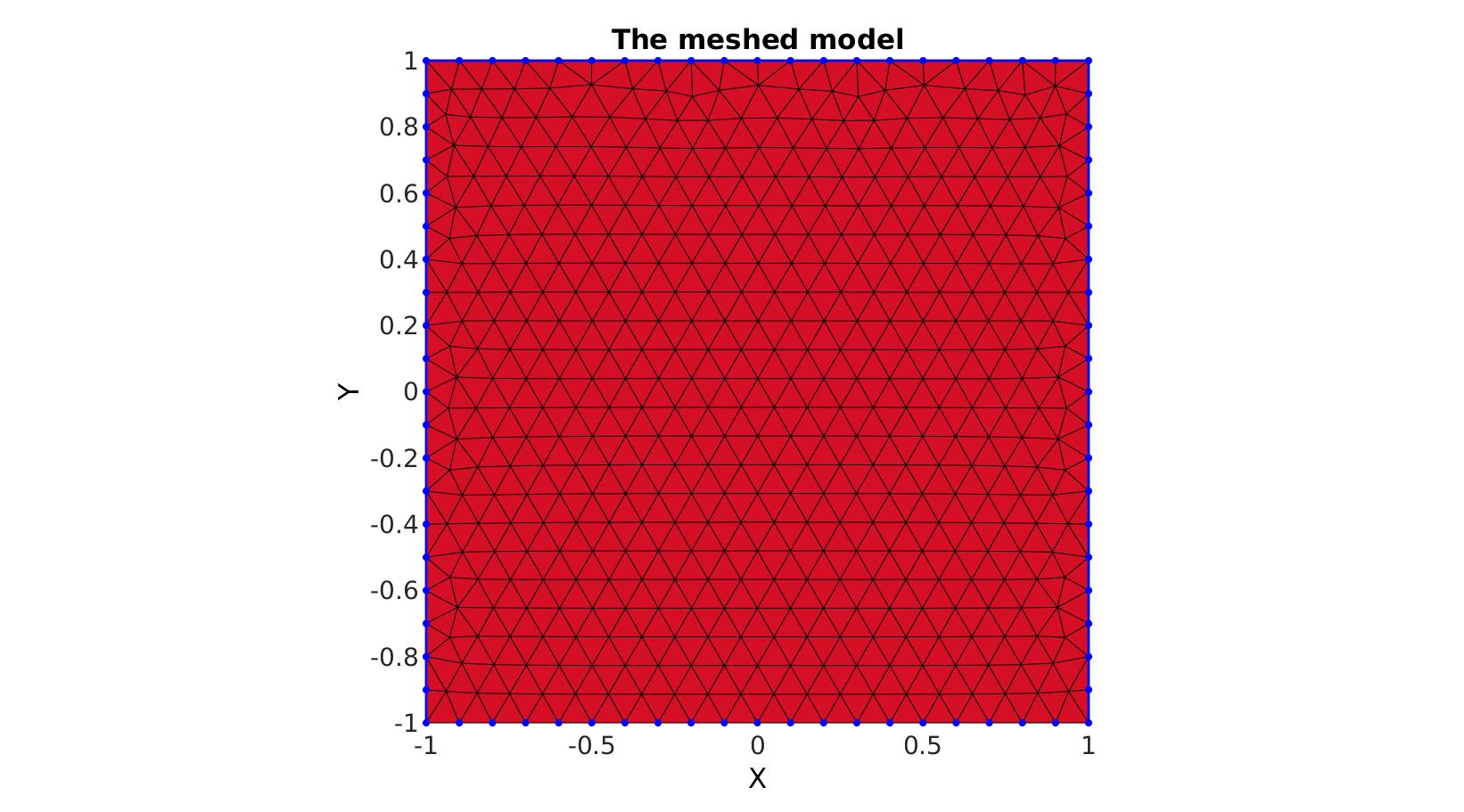
Meshing a 2D region defined by a single boundary curve

Creating boundary curves

V1=[-1 -1; -1 1; 1 1; 1 -1];

Meshing the region

% The input variable regionCell is a cell array containing all the boundary
% curves, e.g. for a two curve region 1 we would have something like
% regionSpec{1}={V1,V2} where V1 and V2 are the boundary curves. Multiple
% curves may be given here. The first curve should form the outer boundary
% of the entire region, the curves that follow should define holes inside
% this boundary and the space inside them is therefore not meshed.

%Defining a region
regionCell={V1}; %A region between V1 and V2 (V2 forms a hole inside V1)
plotOn=1; %This turns on/off plotting
pointSpacing=0.1; %Desired point spacing
resampleCurveOpt=1; %Option to turn on/off resampling of input boundary curves

[F,V]=regionTriMesh2D(regionCell,pointSpacing,resampleCurveOpt,plotOn);
plotV(V1,'b-','LineWidth',2);
axis tight;
drawnow;

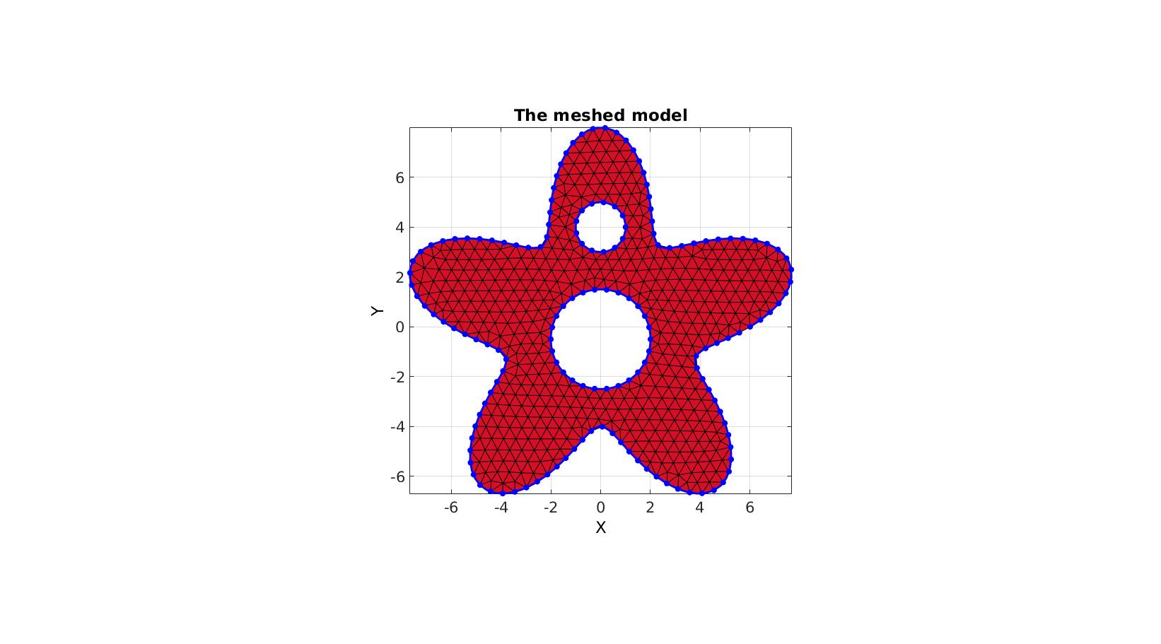
Meshing regions containing holes

Creating boundary curves

%Boundary 1
ns=150;
t=linspace(0,2*pi,ns+1);
t=t(1:end-1);
r=6+2.*sin(5*t);
[x,y] = pol2cart(t,r);
V1=[x(:) y(:)];

%Boundary 2
[x,y] = pol2cart(t,ones(size(t)));
V2=[x(:) y(:)+4];

%Boundary 3
[x,y] = pol2cart(t,2*ones(size(t)));
V3=[x(:) y(:)-0.5];

Meshing the region

% The input variable regionCell is a cell array containing all the boundary
% curves, e.g. for a two curve region 1 we would have something like
% regionSpec{1}={V1,V2} where V1 and V2 are the boundary curves. Multiple
% curves may be given here. The first curve should form the outer boundary
% of the entire region, the curves that follow should define holes inside
% this boundary and the space inside them is therefore not meshed.

%Defining a region
regionCell={V1,V2,V3}; %A region between V1 and V2 (V2 forms a hole inside V1)
plotOn=1; %This turns on/off plotting
pointSpacing=0.5; %Desired point spacing
resampleCurveOpt=1; %Option to turn on/off resampling of input boundary curves

[F,V]=regionTriMesh2D(regionCell,pointSpacing,resampleCurveOpt,plotOn);

plotV(V1,'b-','LineWidth',2);
plotV(V2,'b-','LineWidth',2);
plotV(V3,'b-','LineWidth',2);
axisGeom; view(2);
drawnow;

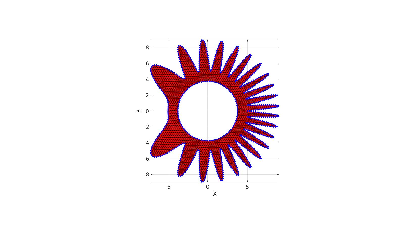
Using input structure instead

Creating boundary curves

%Boundary 1
ns=500;
t=linspace(0,2*pi,ns+1);
t=t(1:end-1);
r=5;
a=2;
R=r-(a.*cos(7*(t-pi).^2)-a);
[x,y] = pol2cart(t,R);
V1=[x(:) y(:)];

%Boundary 2
[x,y] = pol2cart(t,(0.75*r)*ones(size(t)));
V2=[x(:) y(:)];

Meshing the region

%Defining input structure
inputStructure.regionCell={V1,V2};
inputStructure.pointSpacing=0.25;
inputStructure.resampleCurveOpt=1;
inputStructure.plotOn=0;

[F,V,boundaryInd]=regionTriMesh2D(inputStructure);

cFigure; hold on;
gpatch(F,V,'r');
plotV(V(boundaryInd,:),'b.','markerSize',15);
axisGeom; view(2);
drawnow;

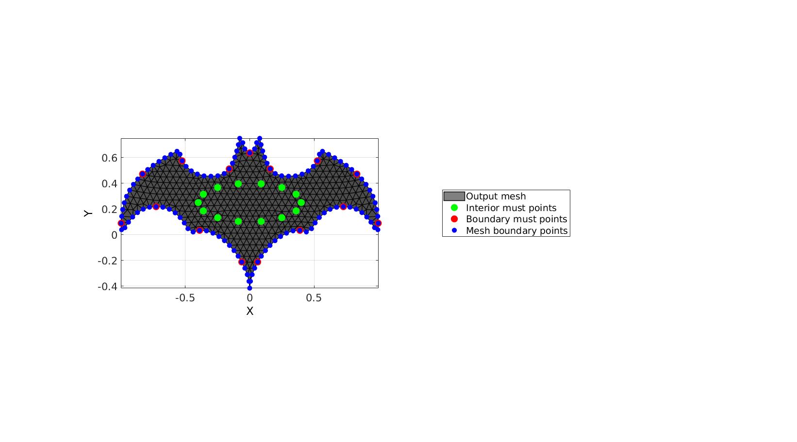
Using must points in the interior and/or boundary, example 1

% Create example boundary curve
V=batman(150);

% Create example interior points
t=linspace(0,2*pi,15)'; t=t(1:end-1);
Vm=[0.4*cos(t) 0.15*sin(t)+0.25];

inputStructure.regionCell={V};
inputStructure.pointSpacing=0.05;
inputStructure.resampleCurveOpt=1;
inputStructure.plotOn=0;
inputStructure.mustPointsInner=Vm;
inputStructure.mustPointsBoundary=V(1:10:end,:);
inputStructure.smoothIterations=250;

[F,V,boundaryInd,indMustPointsInner,indMustPointsBoundary]=regionTriMesh2D(inputStructure);

cFigure; hold on;
hp(1)=gpatch(F,V,'kw','k',1,1);
hp(2)=plotV(V(indMustPointsInner,:),'g.','markerSize',35);
hp(3)=plotV(V(indMustPointsBoundary,:),'r.','markerSize',35);
hp(4)=plotV(V(boundaryInd,:),'b.','markerSize',25);
legend(hp,{'Output mesh','Interior must points','Boundary must points','Mesh boundary points'},'Location','EastOutSide');
axisGeom;
camlight headlight;
view(2)
drawnow;

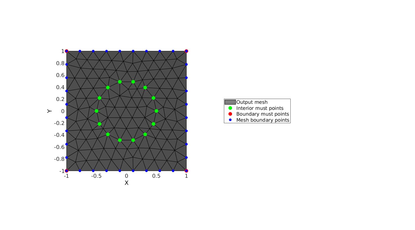
Using must points in the interior and/or boundary, example 2

% Creating boundary curves
V1=[-1 -1; -1 1; 1 1; 1 -1];

% Create example interior points
t=linspace(0,2*pi,15)'; t=t(1:end-1);
Vm=[0.5*cos(t) 0.5*sin(t);];

% Meshing the region

%Defining a region
regionCell={V1}; %A region between V1 and V2 (V2 forms a hole inside V1)
plotOn=1; %This turns on/off plotting
pointSpacing=0.1; %Desired point spacing
resampleCurveOpt=1; %Option to turn on/off resampling of input boundary curves

inputStructure.regionCell=regionCell;
inputStructure.pointSpacing=0.2;
inputStructure.resampleCurveOpt=1;
inputStructure.plotOn=0;
inputStructure.mustPointsInner=Vm;
inputStructure.mustPointsBoundary=V1;
inputStructure.smoothIterations=250;

[F,V,boundaryInd,indMustPointsInner,indMustPointsBoundary]=regionTriMesh2D(inputStructure);

cFigure; hold on;
hp(1)=gpatch(F,V,'kw','k',1,1);
hp(2)=plotV(V(indMustPointsInner,:),'g.','markerSize',35);
hp(3)=plotV(V(indMustPointsBoundary,:),'r.','markerSize',35);
hp(4)=plotV(V(boundaryInd,:),'b.','markerSize',25);
legend(hp,{'Output mesh','Interior must points','Boundary must points','Mesh boundary points'},'Location','EastOutSide');
axisGeom;
camlight headlight;
view(2)
drawnow;

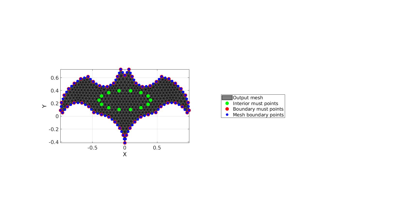
Using must points in the interior and/or boundary, example 3

This example features must points on all boundary points and curve resampling

% Create example boundary curve
V1=batman(50);

% Create example interior points
t=linspace(0,2*pi,15)'; t=t(1:end-1);
Vm=[0.4*cos(t) 0.15*sin(t)+0.25];

inputStructure.regionCell={V1};
inputStructure.pointSpacing=0.05;
inputStructure.resampleCurveOpt=1; %Turn on/off curve resampling
inputStructure.plotOn=0;
inputStructure.mustPointsInner=Vm;
inputStructure.mustPointsBoundary=V1; %Hold on to all boundary points
inputStructure.smoothIterations=250;

[F,V,boundaryInd,indMustPointsInner,indMustPointsBoundary]=regionTriMesh2D(inputStructure);

cFigure; hold on;
hp(1)=gpatch(F,V,'kw','k',1,1);
hp(2)=plotV(V(indMustPointsInner,:),'g.','markerSize',35);
hp(3)=plotV(V(indMustPointsBoundary,:),'r.','markerSize',35);
hp(4)=plotV(V(boundaryInd,:),'b.','markerSize',25);
legend(hp,{'Output mesh','Interior must points','Boundary must points','Mesh boundary points'},'Location','EastOutSide');
axisGeom;
camlight headlight;
view(2)
drawnow;

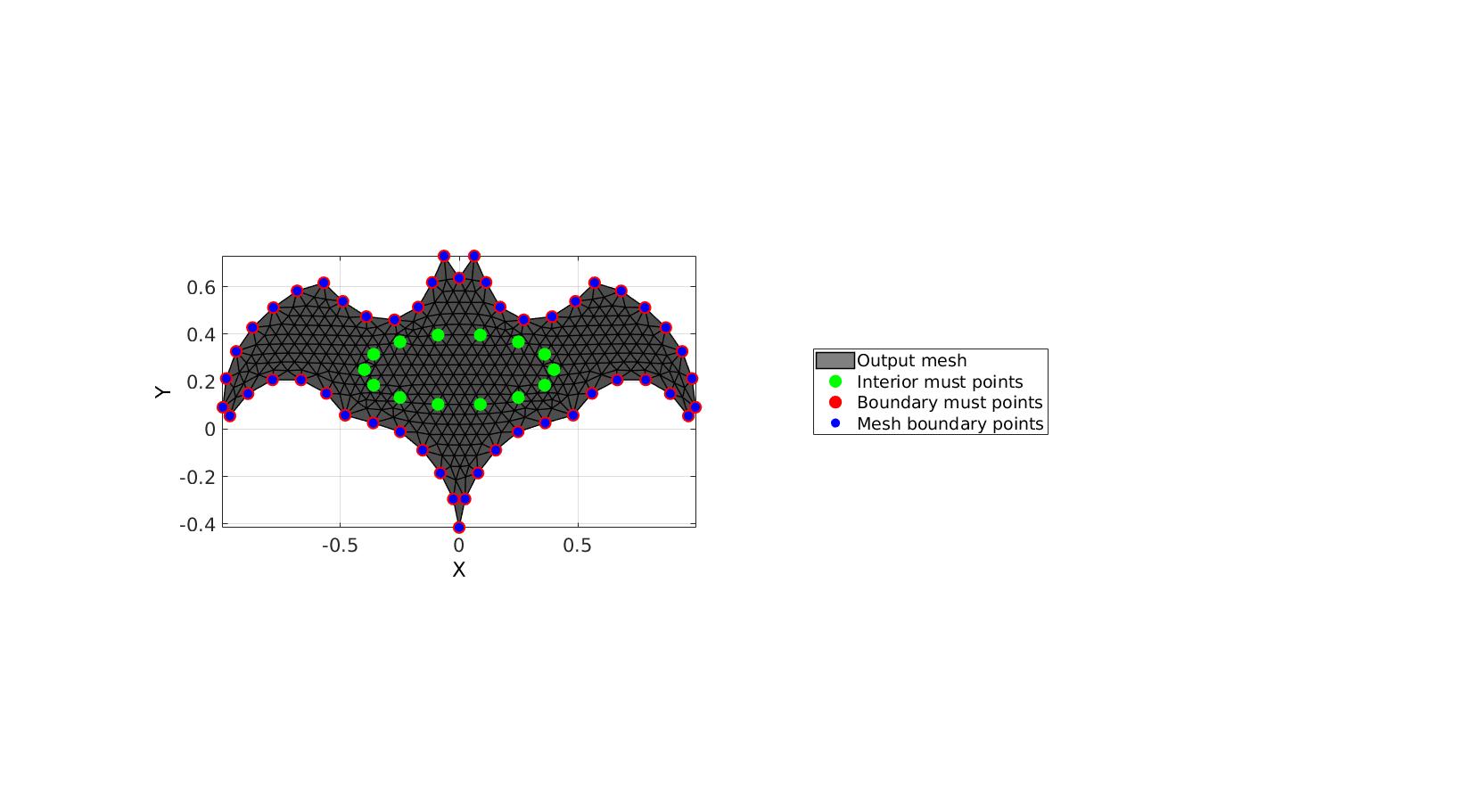
Using must points in the interior and/or boundary, example 4

This example features must points on all boundary points and no curve resampling

% Create example boundary curve
V1=batman(50);

% Create example interior points
t=linspace(0,2*pi,15)'; t=t(1:end-1);
Vm=[0.4*cos(t) 0.15*sin(t)+0.25];

inputStructure.regionCell={V1};
inputStructure.pointSpacing=0.05;
inputStructure.resampleCurveOpt=0; %Turn on/off curve resampling
inputStructure.plotOn=0;
inputStructure.mustPointsInner=Vm;
inputStructure.mustPointsBoundary=V1; %Hold on to all boundary points
inputStructure.smoothIterations=250;

[F,V,boundaryInd,indMustPointsInner,indMustPointsBoundary]=regionTriMesh2D(inputStructure);

cFigure; hold on;
hp(1)=gpatch(F,V,'kw','k',1,1);
hp(2)=plotV(V(indMustPointsInner,:),'g.','markerSize',35);
hp(3)=plotV(V(indMustPointsBoundary,:),'r.','markerSize',35);
hp(4)=plotV(V(boundaryInd,:),'b.','markerSize',25);
legend(hp,{'Output mesh','Interior must points','Boundary must points','Mesh boundary points'},'Location','EastOutSide');
axisGeom;
camlight headlight;
view(2)
drawnow;

GIBBON www.gibboncode.org

Kevin Mattheus Moerman, [email protected]

GIBBON footer text

License: https://github.com/gibbonCode/GIBBON/blob/master/LICENSE

GIBBON: The Geometry and Image-based Bioengineering add-On. A toolbox for image segmentation, image-based modeling, meshing, and finite element analysis.

Copyright (C) 2019 Kevin Mattheus Moerman

This program is free software: you can redistribute it and/or modify it under the terms of the GNU General Public License as published by the Free Software Foundation, either version 3 of the License, or (at your option) any later version.

This program is distributed in the hope that it will be useful, but WITHOUT ANY WARRANTY; without even the implied warranty of MERCHANTABILITY or FITNESS FOR A PARTICULAR PURPOSE. See the GNU General Public License for more details.

You should have received a copy of the GNU General Public License along with this program. If not, see http://www.gnu.org/licenses/.

GIBBON footer text

License: https://github.com/gibbonCode/GIBBON/blob/master/LICENSE

GIBBON: The Geometry and Image-based Bioengineering add-On. A toolbox for image segmentation, image-based modeling, meshing, and finite element analysis.

Copyright (C) 2006-2020 Kevin Mattheus Moerman

This program is free software: you can redistribute it and/or modify it under the terms of the GNU General Public License as published by the Free Software Foundation, either version 3 of the License, or (at your option) any later version.

This program is distributed in the hope that it will be useful, but WITHOUT ANY WARRANTY; without even the implied warranty of MERCHANTABILITY or FITNESS FOR A PARTICULAR PURPOSE. See the GNU General Public License for more details.

You should have received a copy of the GNU General Public License along with this program. If not, see http://www.gnu.org/licenses/.

Published with MATLAB® R2020a